import tequila as tq
from numpy import pi, eye

geometry = """
H 0.0 0.0 0.0
H 0.0 0.0 1.5
H 0.0 0.0 3.0
H 0.0 0.0 4.5
"""

mol = tq.Molecule(geometry=geometry, basis_set="sto-3g")
# switch to native orbitals
# in this case: orthonormalized sto-3g orbitals
mol = mol.use_native_orbitals()
H = mol.make_hamiltonian()
exact = mol.compute_energy("fci")Physical insights into the construction of quantum circuits.
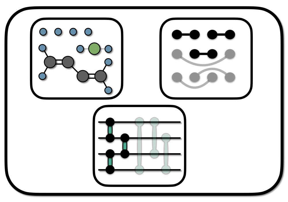
Chemical graphs are a powerful abstraction concept, that allows the qualitative prediction of molecular properties or reactions from a remarkably simple structure. Applied to the design of quantum circuits for electronic ground states (the ground states of molecules), chemical graphs allow physical insight into construction, optimization, and interpretation of quantum circuits.
A detailed description of this methodology is given in arxiv:2207.12421. In this blog entry we will try to approach this circuit design principle through an explicit example. We will use tequila, which has been introduced in other blog entries
Basic Building Blocks
In conventional methodologies of (unitary) coupled-cluster, the wavefunction is generated by exciting electrons from an initial basis state containing a specific number of electrons. A significant distinction between traditional coupled cluster (both unitary and non-unitary) and recent advancements in quantum circuit design lies in the exclusion of higher-order excitations. Instead, the focus is on utilizing a limited set of unitary operations, which are subsequently iteratively applied in a layer-by-layer manner.
Within conventional coupled-cluster approaches, a particular type of excitation, such as a single-electron excitation between two orbitals, is typically accounted for only once. To enhance accuracy, higher-order excitations are introduced.
However, in the context of quantum circuit designs, like the one being discussed, this specific excitation might occur multiple times in various sections of the circuit, while the inclusion of higher-order excitations is often bypassed or minimized.
A simple choice of two basic building blocks for electronic quantum circuits are:
- Orbital Rotations (single electron excitations)
- Pair Excitations (restricted double excitations)
these operations are for example used in the prominent k-UpCCGSD approach or the separable pair approximation.
Take for example two orbitals \(\phi_0\) and \(\phi_1\) encoded into four qubits (\(\phi_0^\uparrow,\phi_0^\downarrow,\phi_1^\uparrow,\phi_1^\downarrow\)) indicating the occupation of the corresponding spin-orbital. The qubit state holding a spin-paired electron pair in orbital \(\phi_0\) is then \[ \lvert 1100 \rangle. \] If we excite this spin-paired electron into the second spatial orbital we end up with \[ \lvert 1100 \rangle \rightarrow \lvert 0011 \rangle. \]
We can treat the spin-paired electrons bound to the same orbital as a quasi-particle – so-called Hard-core Bosons. A wavefunction constructed from Hard-core Boson states entirely is not invariant to rotations in the underlying orbital basis, as we are confining the spin-paired electrons to occupy a specific choice of orbitals. Graphically we can depict this as
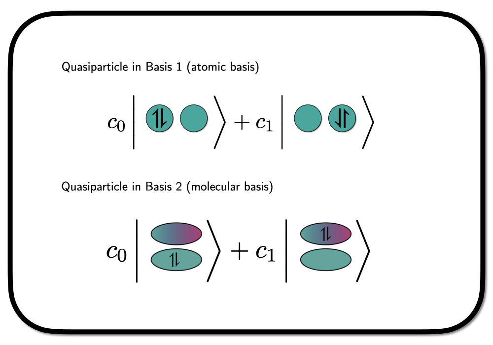
where we have shown the situation in a hydrogen molecule in a minimal basis – one atomic orbital on each hydrogen atom. In this case, the rotation into a different orbital basis clearly leads to a different wavefunction.
The two bases depicted in the figure above are an atomic basis (native orbitals), which we will denote as \(\phi_L\) and \(\phi_R\) for left and right, and a molcular basis \[
\phi_\pm = \frac{1}{\sqrt{2}} \phi_L \pm \phi_R.
\] The state in the molecular basis as depicted above, can now be writte as \[
\lvert \Psi \rangle = c_0 a^\dagger_{+_{\downarrow}} a^\dagger_{+_{\uparrow}} \lvert \rangle + c_1 a^\dagger_{-_{\downarrow}}a^\dagger_{-_{\uparrow}} \lvert \rangle
\] using second quantized language. This is a Hardcore-Boson state with one quasi-particle in two possible orbitals. Expressed in the atomic basis ($ a^{{}} = (a^{L{}} a^{R{}} )$i) this state looks lile \[
\lvert \Psi \rangle = \frac{1}{2} \left(c_0+c_1\right) \left(a^\dagger_{L_{\downarrow}}a^\dagger_{L_{\uparrow}} + a^\dagger_{L_{\downarrow}}a^\dagger_{L_{\uparrow}} \right)\lvert \rangle + \frac{1}{2}\left(c_0-c_1\right) \left(a^\dagger_{L_{\downarrow}}a^\dagger_{R_{\uparrow}} + a^\dagger_{R_{\downarrow}}a^\dagger_{L_{\uparrow}} \right)\lvert \rangle,
\] with an ionic (both electrons either in \(L\) or \(R\)) and a neutral (one electron in \(L\) and one in \(R\)) part. Depending on the choice of the coefficients we can isolate both extremes. In the article this is used to demonstrate how a Hard-core Boson model, with electron pairs confined to the same orbital, is still able to describe bond breaking – i.e. by chosing \(c_1=-c_0\) in the wavefunction above.
Quasi-particle models like the Hard-core Boson approach are therefore dependent on the chosen orbital basis. We can optimize the basis in order to find the best choice for a given quasi-particle wavefunction. These optimizations are however sensitive to initial guesses. Here, molecular graphs serve as a guiding heuristic to initialize good initial guesses for the orbital optimizer. In the original article, this is illustrated in detail on some examples. In the next section, you will find the code for the linear H\(_4\) molecule.
Within quantum circuits, we can rotate the orbital basis with the second building block: the orbital rotations. This allows us to connect several quasi-particle models in sequence by rotating into different bases, correlating the quasi-particles in that basis and finally rotating back to the initial basis.
The molecular graph will take the role as a guiding heuristic helping with placing and initializing the orbital rotation gates as well as the quasi-particle correlators within the quantum circuit.
Example
In the article the linear H4 system has been used to illustrate the construction of quantum circuits from chemical graphs. We will use the H4 example from the paper and provide the code that reproduces it. First we initialize the molecule and represent the Hamiltonian in a minimal basis. Note that we are using (orthonormalized) atomic orbitals as our second quantized basis and not canonical Hartree-Fock orbitals.
As initial state we can construct an SPA circuit using the first graph in the figure above. In this first graph, the H\(_4\) molecule is interpreted as two H\(_2\) molecules. We initializing the graph, by assigning basis orbitals to the vertices. Here we have 4 basis orbitals (atomic s-type orbitals located on the individual atoms), so the assignment is straightforward.
# graph is
# H--H  H--H
graph = [(0,1),(2,3)]
USPA = mol.make_ansatz(name="SPA", edges=graph)
ESPA = tq.ExpectationValue(H=H, U=USPA)
result = tq.minimize(ESPA, silent=True)

print("SPA/Atomic error: {:+2.5f}".format(result.energy-exact))
SPA/Atomic error: +1.09885we see, that the SPA does not perform well – the reason is that we are currently in an atomic orbital basis. In order to rotate the basis, we add orbital rotations to the initial circuit. Here we will use a static angle that will mix the orbitals in a equally weighted fashion (corresponding to Eq.19 in the article, here explicitly represented with unitary circuits). This represents the SPA in a basis that would correspond to the optimized setting in two isolated H2 molecules (i.e. the first graph)
UR0 = tq.QCircuit()
for edge in graph:
    UR0 += mol.UR(edge[0],edge[1],angle=pi/2)

U0 = USPA + UR0
E0 = tq.ExpectationValue(H=H, U=U0)
result = tq.minimize(E0, silent=True)

print("SPA/Molecular error: {:+2.5f}".format(result.energy-exact))
SPA/Molecular error: +0.04009The error is now 40 millihartree. We can bring it further down by allowing the orbitals to relax which can be achieved by adding more orbital rotations with variable angles. We initialize the angles to zero (i.e. we are starting from our previous result as guess). We chose the same pattern as in the \(U_\text{RR}\) circuits in the article
Code
URR0 = mol.UR(0,1,angle="b")
URR0 = mol.UR(2,3,angle="b")
URR0 = mol.UR(1,2,angle="a")

U0 = USPA + URR0 + UR0 + URR0
E0 = tq.ExpectationValue(H=H, U=U0)
result = tq.minimize(E0, silent=True, initial_values=result.variables)

print("SPA/Relaxed-Molecular error: {:+2.5f}".format(result.energy-exact))
SPA/Relaxed-Molecular error: +0.03560Alternatively we can optimize the orbitals with respect to the SPA wavefunction (the strategy from the article) and use this as our orbital basis. As the SPA wavefunction is entirelty within the Hardcode-boson quasiparticle approximation, we can perform the optimization within that approximation reducing our simulation time significantly (see code in the article for the equivalent optimization without HCB approximation)
Code
UHCB = mol.make_ansatz(name="HCB-SPA", edges=graph)
guess = eye(4)
guess[0] = [1, 1,0, 0]
guess[0] = [1,-1,0, 0]
guess[0] = [0, 0,1, 1]
guess[0] = [0, 0,1,-1]
opt = tq.chemistry.optimize_orbitals(circuit=UHCB,molecule=mol, use_hcb=True, initial_guess=guess.T, silent=True)

# update our Hamiltonian
mol = opt.molecule
H = mol.make_hamiltonian()

USPA = UHCB + mol.hcb_to_me()
E = tq.ExpectationValue(H=H, U=USPA)
result = tq.minimize(E, silent=True)

print("SPA/opt-orbitals error: {:+2.5f}".format(result.energy-exact))
SPA/opt-orbitals error: +0.01626Note, that we can get the same result by providing enough orbital rotations to our circuit.
To improve on the SPA model in the optimal basis we take the second graph and apply the following pattern \[ U_G = U_R^\dagger U_C U_R \] that corresponds to 1. rotate into a new orbital basis that resembles the graph structure 2. correlate the quasi particles in this orbital basis 3. rotate back
In the following we will do this for the H4 system using the two graphs indicated in the picture above. The first graph is used for the SPA initalization, and the second graph will add further correlation to the initial SPA state. Note that we included an approximation by neglecting one edge in the second graph which we will not correlated. The code-block is identical as the on in the appendix of the article.
Code
# dependencies: tequila >= 1.8.7, pyscf~=1.7, scipy~=1.7
# suggested quantum backend for optimal performance: qulacs >= 0.3
import tequila as tq
from numpy import eye, pi

# Create the molecule object
# use orthonormalized atomic orbitals as basis
geometry = "h 0.0 0.0 0.0\nh 0.0 0.0 1.5\nh 0.0 0.0 3.0\nh 0.0 0.0 4.5"
mol = tq.Molecule(geometry=geometry, basis_set="sto-3g")
energies = {"FCI":mol.compute_energy("fci")}
# switch from canonical HF orbitals to orthonormalized STO-3G orbitals
# to follow notation in the article
mol = mol.use_native_orbitals()

# Create the SPA circuit for
# Graph: H -- H    H -- H
# edges get tuples of orbital-indices assigned
USPA = mol.make_ansatz(name="SPA", edges=[(0,1),(2,3)])

# initial guess for the orbitals
# according to graph in Eq.(17) and orbitals in Eq.(19)
guess = eye(4)
guess[0] = [1.0,1.0,0.0,0.0]
guess[1] = [1.0,-1.,0.0,0.0]
guess[2] = [0.0,0.0,1.0,1.0]
guess[3] = [0.0,0.0,1.0,-1.]

# optimize orbitals and circuit parameter
# PySCF interface
opt = tq.chemistry.optimize_orbitals(mol, circuit=USPA, initial_guess=guess.T)
print("Optimized Orbital Coefficients")
print(opt.molecule.integral_manager.orbital_coefficients)
energies["SPA"] = opt.energy

# get Hamiltonian with optimized orbitals
H = opt.molecule.make_hamiltonian()

# initialize rotations to graph in Eq.(21)
# H    H -- H    H
# as illustrated in Eq.(24)
# UR as in Eq.(7) uses spatial orbital indices
R0 = tq.Variable("R0")
R1 = tq.Variable("R1")
UR0 = mol.UR(0,1,angle=(R0+0.5)*pi)
UR0+= mol.UR(2,3,angle=(R0+0.5)*pi)
UR1 = mol.UR(1,2,angle=(R1+0.5)*pi)

# initialize correlator according to Eq.(22)
UC = mol.UC(1,2,angle="C")

# construct the circuit for both graphs
U = USPA + UR0 + UR1 + UC + UR1.dagger() + UR0.dagger()
# optimize the energy
E = tq.ExpectationValue(H=H, U=U)
result = tq.minimize(E, silent=True)
energies["SPA+"] = result.energy
print(energies)
Code
for k,v in energies.items():
    if "fci" in k.lower(): continue
    print("{:5} error : {:+2.5f}".format(k,v-exact))
SPA error : +0.01626
SPA+ error : +0.00844Further Reading
Dependencies and Installation
In order to execute code from this blog entry you need the following dependencies in your environment
pip install tequila-basic
pip install pyscf
# optional (significantly faster)
pip install qulacs