import tequila as tq

geometry = "Be 0.0 0.0 0.0"
mol = tq.Molecule(geometry=geometry, basis_set="6-31G")

c,h,g = mol.get_integrals(two_body_oderings="mulliken")
converged SCF energy = -14.5667640335096What are electronic Hamiltonians and how can we construct them?
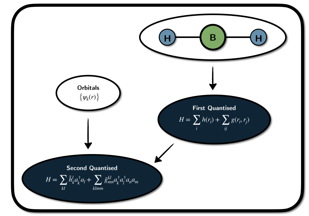
First Quantized Formulation:
Second Quantized Formulation:
The word molecule often stands for \(N_\text{e}\) electrons with coordinates \(r_k\) moving in a potential created by atomic nuclei - assumed to be fixed point-charges with coordinates \(R_A\) and charges \(N_A\). The electronic Hamiltonian is then the operator expressing the interactions of the electrons in that potential \[H = \sum_{k}^{N_\text{e}} h\left(r_k\right) + \sum_{k}^{N_\text{e}} \sum_{l<k} g\left(r_k,r_l\right) + V_\text{nn}.\] We write it three parts and a constant, which are in atomic units:
With this, we have fully defined it, and the lowest eigenvalue of this differential operator gives the corresponding ground state energy. To ensure that the ground state describes a multi-electron system, we must impose restrictions on the wavefunction - Fermions have a spin and anti-symmetric permutation symmetry.
As we are describing electrons, they need to obey fermionic antisymmetry. In first quantization (or real-space formulation), the Hamiltonian does not have that property included, so without restrictions on the wavefunctions, it only describes \(N_\text{e}\) negatively charged point-particles without any permutation symmetries or spin.
We can add spin conveniently by defining a single-electron wavefunction as a so called spin-orbital: A three-dimensional function \(\psi(r) \in \mathcal{L}^2(\mathbb{R}^3)\), describing the electron in spatial space, augmented with a spin-state \[\lvert\sigma\rangle \in \text{Span}\left\{\lvert \uparrow \rangle, \lvert \downarrow \rangle\right\} \equiv \mathbb{C}^2.\] If the set of spatial orbitals \(\psi_k\) forms a complete basis in \(\mathcal{L}^2(\mathbb{R}^3)\), we have an exact description of the electron. A convenient notation is to express the spin component as a function of a spin-coordinate \(s\left\{-1,1\right\}\) and combine spin coordinate \(s\) and spatial coordinate \(r\) to \(x=(r,s)\). In a given set of \(M\) spatial orbital, an arbitrary one electron wavefunction can then be expressed as \[ \Psi(x) = \sum_k^{2M} c_k \phi(x) = \sum_{l}^{M} \psi_{l}(r)\otimes \left( c_{2l}\lvert \uparrow \rangle + c_{2l+1} \lvert \downarrow \rangle \right) \] with the spin-orbitals defined as \[ \phi_k = \psi_{\lfloor{i/2}\rfloor} \otimes \lvert \sigma(k) \rangle,\; \sigma_k=\begin{cases} \lvert \uparrow \rangle,\; k \text{ is even} \\ \lvert \uparrow \rangle,\; k \text{ is odd} \end{cases}. \] Many electron functions can then be constructed as linear combinations of anti-symmetric products of single electron functions (so called Slater-Determinants). \[ \Psi\left(x_1, \dots, x_{N_\text{e}}\right) = \sum_{m} d_m \det\left(\phi_{m_1},\dots, \phi_{m_{N_\text{e}}}\right) \ \]
Using second quantized language, we can significantly simplify the treatment of electron spin and anti-symmetry with the help of abstract field operators \(\hat{\phi}^\dagger(x)\) (\(\hat{\phi}(x)\)) that create (or annihilate) electrons at spin-position \(x\). With them, we can formaly write the electronic Hamiltonian as \[H = \int \hat{\phi}^\dagger(x) h(x) \hat{\phi}(x) \operatorname{x}x + \int \int \hat{\phi}^\dagger(x)\hat{\phi}^\dagger(y) g(x,y) \hat{\phi}(x)\hat{\phi}(y) \operatorname{d}x\operatorname{d}y+ V_\text{nn}.\] The wavefunction is now only required to carry information about electron occupancies at all points in space. When acting on the wavefunction, the one-body part of the operator is first annihilating an electron at point \(x\). If no electron is present, this will lead to an energy contribution of zero and otherwise invoke \(h(x)\), followed by the restoration of the electron by the creation operator. The two-body part acts in the same way and the integrals ensure that we probe all points in space. In practice, this is unfeasible, and it is convenient to introduce a finite basis in the form of spin orbitals to expand the field operators as \[\hat{\phi}(x) = \sum_k \phi(x)_k a_k, \] leading to the more prominent form of the second quantized Hamiltonian \[ H = \sum_{ij} \tilde{h}^i{j}a^\dagger_i a_j \sum_{ijkl} \tilde{g}^{ij}_{kl} a^\dagger_i a^\dagger_j a_l a_k + V_\text{nn}. \] The new discretized operators \(a^\dagger_k\) (\(a_k\)) are now creating (annihilating) an electron in the spin orbital \(\phi_k\) and the tensors \(\tilde{h}^{i}_{j}\) and \(\tilde{g}^{ij}_{kl}\) are integrals over the one- and two-body operators and the spin orbitals. The one-body integrals are then given by \[ \tilde{h}^{i}_{j} = h^{\lfloor{i/2}\rfloor}_{\lfloor{j/2}\rfloor} \langle \sigma_i \vert \sigma_j \rangle \] with the spatial part \[ h^{k}_{l} = \langle k \rvert h \lvert l \rangle \equiv \int \psi_k^*(r) h(r) \psi_l(r) \operatorname{d}r. \] In the same way, the spatial part of the two-body integrals is given by \[ g^{ij}_{kl} = \langle i j \rvert g_{12} \lvert k l \rangle \equiv \int \int \psi_i^*(r_1) \psi_j^*(r_2) \frac{1}{|r_1-r_2|} \psi_k(r_1) \psi_l(r_2) \operatorname{d}r_1 \operatorname{d}r_2. \] Note that there exist three different short notations \[ \langle ij\vert kl \rangle \equiv \left(ik \vert jl \right) \equiv \left[ ij \vert lk \right] \] usually referred to as Dirac (physicist, 1212), Mulliken (chemist, 1122) and openfermion (google, 1221) notations. Depending on the convention used, the meaning of the indices \(g^{ij}_{kl}\) changes. This is a bit inconvenient, but we can’t change it anymore. Most quantum chemistry packages (pyscf, psi4) use the Mulliken convention, some quantum computing packages adopted the google convention, and the Dirac convention is often found in articles. In the tequila package we tried to automatize most of it away for user convenience. Here is a small example on how to get the integrals using tequila (with either pyscf or psi4 in the back):
import tequila as tq
geometry = "Be 0.0 0.0 0.0"
mol = tq.Molecule(geometry=geometry, basis_set="6-31G")
c,h,g = mol.get_integrals(two_body_oderings="mulliken")converged SCF energy = -14.5667640335096for most applications, the integrals are however processed automatically in the back.
Let’s look at first and second quantized Hamiltonians and wavefunctions in an explicit example: The Helium atom (charge \(N_\text{He}=2\) and nuclear coordinate \(R_\text{He} = (0,0,0)\)) in a basis of two spatial orbitals \(\left\{\psi_0, \psi_1 \right\}\).
For the neutral electron with 2 electrons, the Hamiltonian is:
\[
H(r_1,r_2) = -\frac{\nabla^2}{2} - \frac{\nabla^2}{2} - \frac{2}{\|r_1\|} - \frac{2}{\|r_2\|} + \frac{1}{\|r_1 - r_2 \|}
\] and a general two-electron Slater-determinant is written as
\[
\det\left(\phi_k,\phi_l\right) = \frac{1}{\sqrt{2}} \left( \phi_k(r_1) \phi_l(r_2) - \phi_l(r_1) \phi_k(r_2) \right).
\]
All possible Slater-determinants in the given basis:
closed-shell singlets (both electrons in the same spatial orbital):
\[
\det\left(\phi_0 \phi_1 \right) = \frac{1}{\sqrt{2}}\psi_0(r_1) \psi_0(r_1) \otimes \left( \lvert \downarrow \uparrow \rangle - \lvert \uparrow \downarrow \rangle \right)
\] \[
\det\left(\phi_3 \phi_4\right) = \frac{1}{\sqrt{2}}\psi_1(r_1) \psi_1(r_1) \otimes \left( \lvert \downarrow \uparrow \rangle - \lvert \uparrow \downarrow \rangle \right)
\]
open-shell polarized triplets:
\[
\det\left(\phi_1 \phi_3\right) = \left(\psi_0(r_1) \psi_1(r_2) + \psi_1(r_1) \psi_0(r_2)\right) \otimes \left( \lvert \uparrow \uparrow \rangle \right)
\]
\[ \det\left(\phi_2 \phi_4\right) = \left(\psi_0(r_1) \psi_1(r_2) + \psi_1(r_1) \psi_0(r_2)\right) \otimes \left( \lvert \downarrow \downarrow \rangle \right) \]
A general two-electron wavefunction can then be written as a linear combination of those 6 Determinants (note however, that the different spin-symmetries, i.e. the triplet and the two singlets, usually don’t mix) \[ \Psi(x_1,x_2) = \sum_{i<j\in\left\{0,1\right\}} d_{ij} \det\left(\phi_i\phi_j\right) \] Note how this always denotes a two-electron wavefunction. The electron number directly enters the definition of the first quantized Hamiltonian and therefore defines the space onto which the Hamiltonian acts.
For numerical procedures it is often necessary to directly express the Hamiltonian in the given basis. Here this would mean to compute all matrix elements \[ H_{ij} = \langle \det\left(\phi_m\phi_n\right)\rvert H \lvert \det\left(\phi_k\phi_l\right) \rangle. \] In this two electron example this is no problem, the task of computing all matrix elements will however become unfeasible with growing electron number due to the growth of possible determinants. Explicit computation of the Hamiltonian in the given basis is usually only performed within further approximations - e.g. truncated configuration interaction methods that only include slater determinants that differ in a specific number of orbitals from a given reference determinant.
In second quantization it is sufficient to compute the one- and two-body integrals given above to define the Hamiltonian. They grow with the fourth power of the basis size rendering the task always feasible.
A general wavefunction can be constructed from all possible linear combinations of electronic configurations in the given spin-orbital basis - denoted by so called occupation vectors representing which spin orbitals are occupied and not. In this case we have 4 spin orbitals then therefore \(2^4=16\) different configurations:
vacuum
\[\langle 0000 \rangle\]
single electron
\[
\lvert 1000 \rangle, \vert 0100 \rangle, \lvert 0010 \rangle, \lvert 0001\rangle,
\]
two electrons
\[
\lvert 1100 \rangle, \lvert 0011 \rangle, \lvert 1001 \rangle, \lvert 0110 \rangle, \lvert 1010\rangle, \lvert 0101 \rangle,
\]
three electrons
\[
\lvert 1110 \rangle, \lvert 1101 \rangle, \lvert 1011 \rangle, \lvert 0111 \rangle,
\]
four-electrons
\[
\lvert 1111 \rangle.
\]
A general wavefunction is then given by
\[\lvert \Psi \rangle = \sum_{k=0}^{16} c_k \lvert \text{binary}(k) \rangle.\]